
Summary
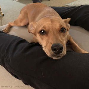
I came up with this project as a fun way to get hands-on experience with tensorflow and certain techniques that are specific to machine learning. The goal I set for myself was to train a Generative Adversarial Network (GAN) to produce photorealistic fake images of Honey the dog.
I begin this post with a brief introduction to the GAN and a look at the training data. Then, I give a walk-through of the two attempts I made, starting with background of the respective architecture and concluding with the result. The sidenotes serve as a reminder of useful software and procedures I came across while working on this project. Enjoy!
What is a GAN?
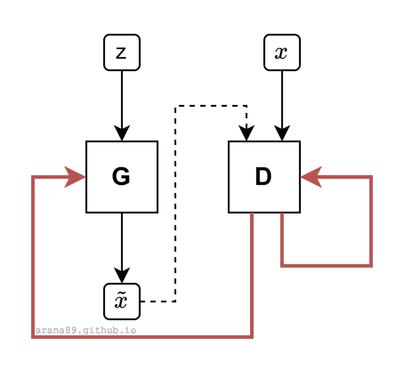
The Generative Adversarial Network1 (GAN) is a type of deep learning architecture that has experienced mainstream exposure due to its simple, yet striking visual demonstrations of the power of modern machine learning. A GAN consists of two independent components, a generator \(G\) and a discriminator \(D\), working collectively to synthesize output that is similar to the training data. The generator is given a random noise input and aims to produce output \(\tilde{x}\) that is statistically indistinguishable from the training data \(x\). The discriminator performs two binary classification tasks – one to identify \(x\) as the real data and the other to identify \(\tilde{x}\) as the output from \(G\). The network is described as adversarial because \(D\) is penalized by inaccurate classification and \(G\) is penalized when \(D\) is able to correctly identify \(\tilde{x}\) as its generated output. The GAN can be more easily explained using the framework of game theory, with the solution existing at the Nash equilibrium of the two loss functions
\[\underset{w^{G}}{\operatorname{argmin}}J_G(w^{D}, ~w^{G})\] \[\underset{w^{D}}{\operatorname{argmin}}J_D(w^{D}, ~w^{G})\]
where each loss \(J\) is a function of the weights of both \(D\) and \(G\).
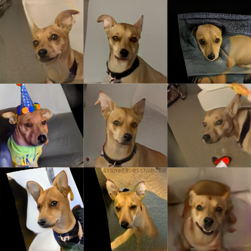
A Look at the Data
The data I would use to train my GAN consist of \(\sim 2000\) images of Honey taken at different stages of life in a variety of settings.
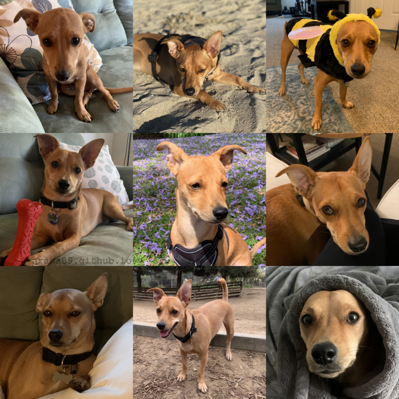
The variety is beneficial in that Honey’s face has been photographed with relatively full coverage, but also presents some interesting challenges from a machine learning perspective. The quality of a trained network generally scales with the size of the training data, and for GANs this is in the neighborhood of \(\sim 1\times 10^5-1\times 10^6\) images. Neural networks are prone to overfit when trained on small datasets. Secondly, the variety in non-critical areas (body, background, orientation, etc.) could have a confounding effect and need to be minimized.
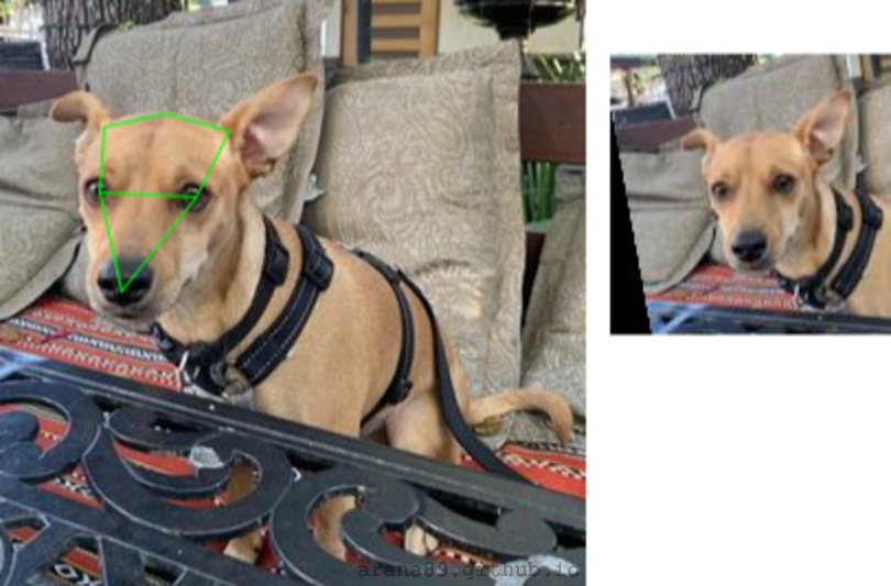
Data Cleaning
For this project, data cleaning entailed the removal of as much non-essential image variance as possible, so that the network would only learn the semantics of Honey’s face. I found dlib, an open source library containing a lot of useful functions for deep learning data processing and analysis. I used a CNN, which had been pre-trained for dog face detection, to output the exact pixel coordinates and relative orientation of Honey’s face in every picture. Then I used extract_image_chip to crop a square region around the face and rotate it such that all images in the dataset had roughly the same in-plane orientation. This procedure also discarded images where the 6 “landmark” facial features – top, left ear, right ear, nose, left eye, right eye – were not visible due to obstruction.
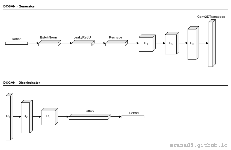
Attempt 1: DCGAN
Architecture
The Deep Convolutional GAN2 (DCGAN) was an early breakthrough architecture that demonstrated GANs could produce high resolution output in a single shot. DCGAN also showed an understanding of semantics by performing simple arithmetic on image attributes. The DCGAN characteristically uses strided convolutions in \(D\) and sub-pixel convolutions in \(G\). Also, batch normalization is used in all layers except the last layer of \(G\) and first layer of the \(D\). The generator uses ReLU activation while the discriminator uses LeakyReLU activation.
Loss Function
Both \(D\) and \(G\) use a binary cross-entropy loss function
\[J = -y~log(\hat{y}) - (1-y)log(1-\hat{y})\]where \(y\) is the probability distribution of the input data and \(\hat{y}\) is the probability distribution of the model. This loss function is a measure of how accurately the discriminator can classify the real images \(D(x) = 1\) and the generated images \(D(\tilde{x}) = 0\). So the discriminator loss function looks like
\[J_{D} = -log(D(x)) - log(1-D(\tilde{x}))\]where \(\tilde{x} = G(z)\). The generator loss function
\[J_{G} = -log(D(\tilde{x}))\]is chosen such that the gradient is small when the generated images are successfully “tricking” the discriminator (when \(D(G(z))\sim 1\)).
DCGAN Results
I built a simple DCGAN as a tf.keras.Model with an output shape of (64,64,3) to keep the computation time reasonable. The training images were resized to match the output dimensions, then scaled layers.Rescaling(scale=1./127.5, offset=-1) and shuffled into minibatches of BATCH_SIZE = 64. The dataset was augmented with random horizontal flips and small brightness perturbations. Both the discriminator and generator used adaptive gradient descent tf.keras.optimizers.Adam with a learning_rate=2e-4. I used tf.train.Checkpoint to limit training to nights when my PC was idle. Training stagnated after about \(24 \) hours of training, producing output that looked like:
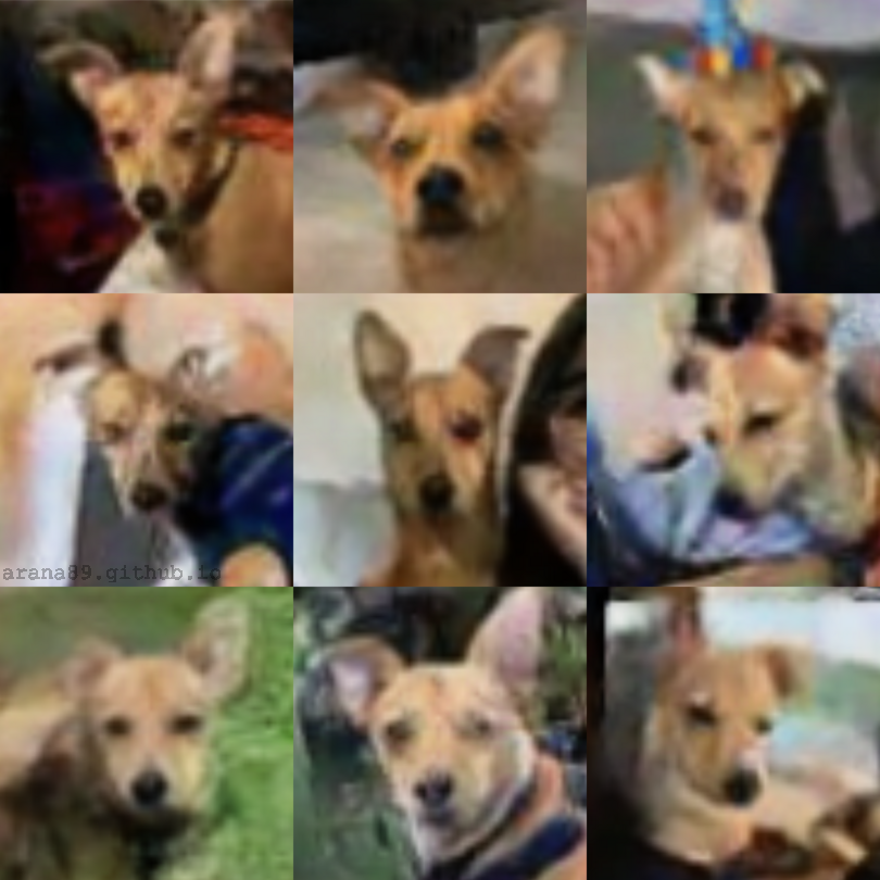
If you squint your eyes and sit far away from your monitor, you may be tricked into thinking the generated images look like the real Honey, but I wasn’t satisfied. My suspicion was that the size of the dataset was a fundamental problem in this approach. So, I continued my literature review – now looking at architectures and methods that specialize in small data.
Sidenote: Docker
I didn’t encounter containerization while in grad school, although it now seems to be gaining popularity in academia. I will be using container orchestration in an upcoming project, so I took this as an opportunity to play around with docker and compare it to virtualenv/venv/pipenv/... for the purpose of dependency control. After downloading the container image
docker pull tensorflow/tensorflow:latest-gpu-jupyter
I had a lightweight, portable jupyter notebook with tensorflow installed. Since I was working on both a desktop and laptop, I kept my working directory on a network drive and passed it to docker as a persistent volume.
docker run -it -v /path/to/working/dir:/tf/notebooks -p 8888:8888 tensorflow/tensorflow:latest-gpu-jupyter
Overall, I think a container is a better option than a virtual environment in this scenario. I view the container as a compromise between a virtual environment and a VM, beating the former in reproducibility and the latter in weight.
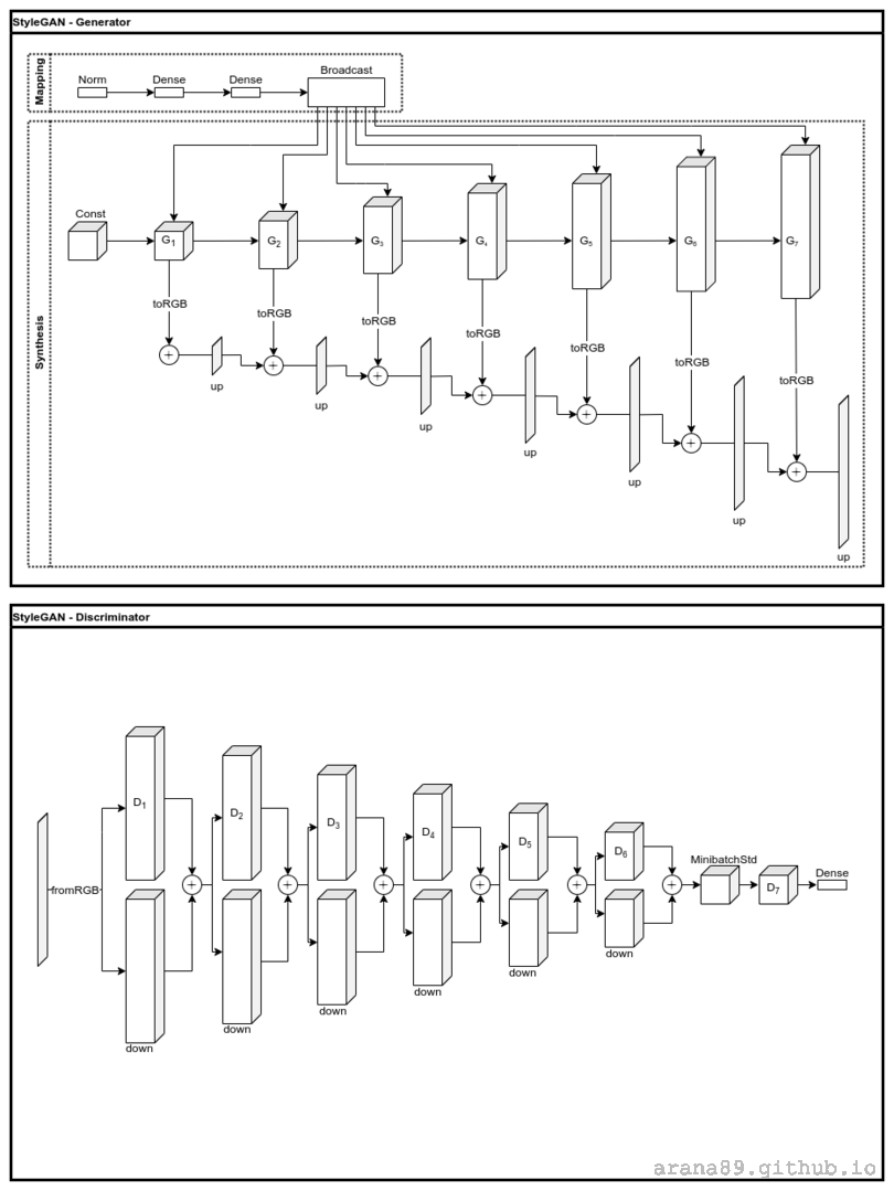
Attempt 2: StyleGAN
Architecture
StyleGAN3 takes a fundamentally different approach compared to DCGAN. While the DCGAN generator takes the input \(z\) directly into the convolution layers, StyleGAN has a more complex generator consisting two distinct sub-networks. The mapping sub-network serves to embed \(z\) into a latent space \(G_{map}(z) = w\). This mapping produces an abstract representation of the spatially invariant features (“styles”) present in the data. The synthesis sub-network \(G_{synth}\) then learns how to scale and bias the styles, and finally combine them to form an output image. The name derives from the techniques used in style transfer4 that inspire the generator architecture. StyleGAN also uses improved augmentation techniques and a modified loss function, described in the following sections.
Loss function
It has been shown that unregularized GAN training is not always convergent, even with extremely small step size5. Regularization is an optimization technique in which terms are added to the loss function to aid in convergence. While regularization and convergence in GAN training is still an open field of study, one effective regularizer is of the form
\[R_1(w^{D}) = \frac{\gamma}{2} \parallel \nabla D_{w^{D}}(x)\parallel^2\]where \(\gamma\) is an adjustable scaling factor. The \(R_1\) regularizer is a gradient penalty acting on the discriminator when it deviates from the Nash equilibrium solution. The StyleGAN loss function used in this project is effectively the same as the DCGAN loss function, with \(R_1\) regularization added to \(J_D\).
Data Augmentation
Data augmentation is a straightforward technique in certain ML applications, such as image classification. When operations that preserve image morphology – rotation, noise, perturbing brightness, contrast etc. – are applied to the dataset, the classifier sees an effectively larger and more diverse dataset and thus learns to better classify the underlying data. However, simple augmentation applied to GANs can result in the generator incorrectly learning to produce augmented images, an undesirable phenomenon known as “augmentation leaking”.
It has been shown6 that a large class of augmentations can be made to be “non-leaking”, that is, not present in the generated output, as long as they are applied to the training data with some probability
\[p_{aug} < 1~.\]The optimal value of \(p_{aug}\) that maximally augments the data without corrupting \(G\) can be determined iteratively within the training loop. I found a marked improvement in the StyleGAN output when this augmentation technique was applied.
Transfer Learning
In theory, neural networks are able to apply training knowledge gained from one dataset to other similar datasets. However, the optimal application of this idea, known as “transfer learning”, is still an open research problem. When done correctly, transfer learning is able to drastically improve convergence and efficiency. In practice, this usually involves choosing a network that has been trained on data which is sufficiently similar to the data of interest and adjusting the gradient step size to be small. Luckily for me, StyleGAN was published with some pre-trained examples, one of which had been trained on dog images…
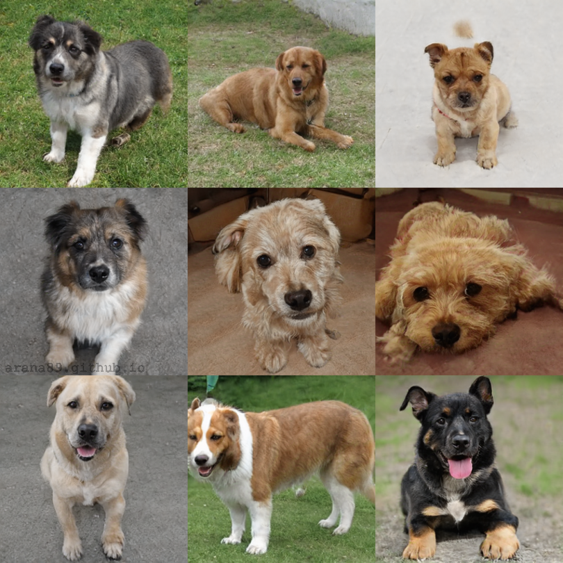
StyleGAN Results
Excited that I might avoid the herculean computation effort of training styleGAN from scratch, I began transfer learning with the pre-trained network described in the previous section. Both \(D\) and \(G\) had a fixed step size learning_rate = 2.5e-3. The regularization weight was set r1_gamma = 0.8192. The augmentation strength is modulated by a chosen heuristic. In this case, tune_heuristic = "rt" monitors the sign of the discriminator output as a measure of overfitting. The augmentation probability is adjusted so the heuristic moves toward a target value, which in this case is tune_target = 0.6. I had no halting criteria other than running out of Google cloud credit the apparent quality of the generator output, which met my arbitrary standards at approximately 6000 iterations.
The quality of the images produced was much improved by using a state-of-the-art network architecture and transfer learning. I suspect that the output quality could be further improved with more extensive background removal in the training data alongside augmentation using images of dogs that are most similar in appearance to Honey – perhaps automated with a classification net.
Sidenote: Google Cloud Platform
Training StyleGAN was above the capability of my local computer, so I took this as a chance to try commercially available cloud computing resources. I went with Google Cloud Platform (GCP) just because they were giving free computation credit to first time users. I also saw a wide variety of VMs available on the compute engine, including many that are configured for deep learning. After setting up the gcloud CLI on my pc, I used
gcloud compute instances create
with the appropriate flags to initialize a Debian based VM that was configured with TF 1.15 and CUDA 11.0. Then, I could SSH to this VM and download the training code and data from my git repo. Once it was up and running, I SSH’d in to pull the code and training data from my git repo, run the training scripts and monitor output. The results shown in the styleGAN section were achieved after training on a Nvidia V100 for \(\sim 36\) hours. In an upcoming project, I plan to utilize Kubernetes.
Special thanks to Daisy for providing all the pictures of Honey!