Summary

Gyms play an important role in the development of the rapidly evolving meta strategy of mixed martial arts (MMA). Motivated by curiosity as a casual fan and hobbyist of the sport, I aggregate and visualize publicly available data to provide insight into gym performance and distribution across California.

Scraping and Tabulating: Pandas and BeautifulSoup

California’s amateur MMA governing body maintains a website with fighter information and bout statistics. Queries are limited to searching for individual fighters.

The data as it is presented on the website of the governing body for amateur MMA in California.

The data exist as a paginated table, making it relatively straightforward to scrape. I used the Pandas function read_html() to scrape and pipe the data directly into a dataframe. It uses BeautifulSoup4 on the back-end, which itself is just a wrapper for a set of html parsers. This loop goes through each page of the table and appends the data to the main dataframe object:

import pandas as pd

page_size = 20 #number of rows per page
row_count = 1
keep_going = True
df = pd.DataFrame()

while keep_going:
    url = f'https://camomma.org/Users-fighters&from={row_count}'
    temp_df = pd.read_html(url)[0]    
    df = pd.concat([df,temp_df])    
    row_count += page_size

    if len(temp_df) == 0:
        keep_going = False

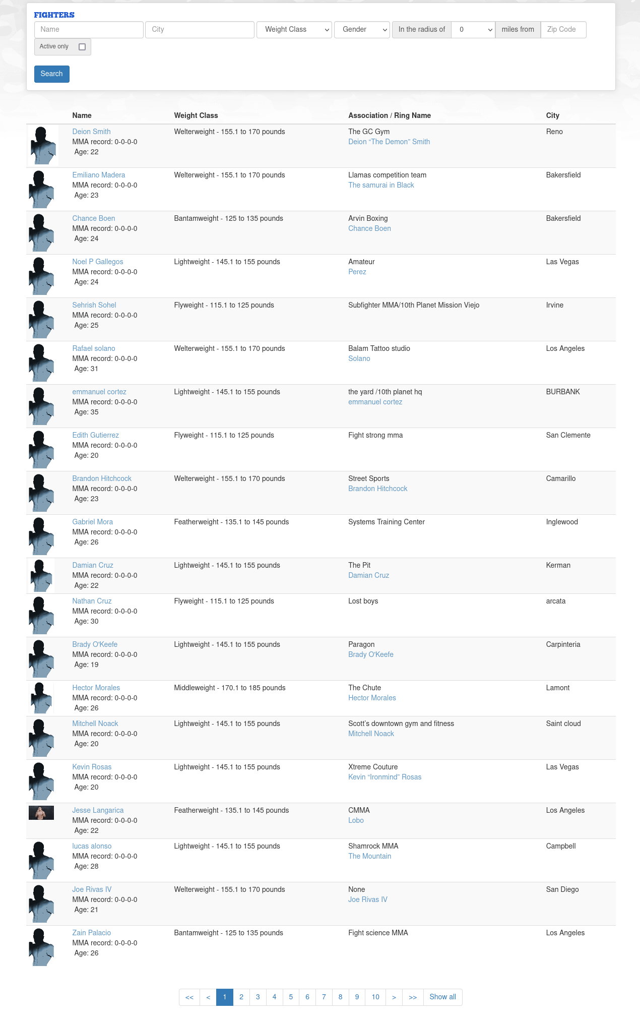
The resulting dataframe contains the fighter’s name, nickname, age, record, weight class, gym association and city:

Name	Weight Class	Association / Ring Name	City
Derrick Ko MMA record: 0-0-0-0 Age: 25	Bantamweight - 125 to 135 pounds	Goon Squad MMADerrick "Cash" Ko	San Francisco
Kaien Cicero MMA record: 0-0-0-0 Age: 20	Lightweight - 145.1 to 155 pounds	None	Brea
Darrian Williams MMA record: 0-0-0-0 Age: 28	Heavyweight - 230.1 to 265 pounds	Samurai Dojo	Exeter
Christian Zubiate MMA record: 0-0-0-0 Age: 25	Welterweight - 155.1 to 170 pounds	10th planetHead Hunter	Newport Beach
Kevin Wright MMA record: 0-0-0-0 Age: 25	Middleweight - 170.1 to 185 pounds	10th PlanetKevin Wright	phoenix

The formatting isn’t quite right, as the Name column also contains the fighter’s record and age. However, this can be fixed with a little bit of regex’ing:

df[['name', 'record', 'age']] = df['Name'].str.extract('(?i)(?P<name>.+?(?=\sMMA))\sMMA\srecord:\s(?P<record>(?<=MMA\srecord:\s)\d+-\d+-\d+-\d+).*?\sAge:\s(?P<age>\d+)', expand=True)
df.pop('Name')

#reorder columns
cols = df.columns.to_list()
cols = cols[-3:] + cols[:-3]
df = df[cols]

Here is a breakdown of the expression:

(?i)(?P<name>.+?(?=\sMMA))\sMMA\srecord:\s(?P<record>(?<=MMA\srecord:\s)\d+-\d+-\d+-\d+).*?\sAge:\s(?P<age>\d+)

(?i) : global case insensitive modifier

(?P<name>.+?(?=\sMMA)) : lazy match everything until reaching 'MMA'

(?P<record>(?<=MMA\srecord:\s)\d+-\d+-\d+-\d+) :  After 'MMA record: ', capture the 4 digits that are separated by dashes

.*?\s : Lazy catch for rows where a pankration/combat grappling record was also listed for a fighter. This data wasn't used.

Age:\s(?P<age>\d+) : Capture the digits after 'Age: '

After the initial formatting, the table looks like:

name	record	age	Weight Class	Association / Ring Name	City
Derrick Ko	0-0-0-0	25	Bantamweight - 125 to 135 pounds	Goon Squad MMADerrick "Cash" Ko	San Francisco
Kaien Cicero	0-0-0-0	20	Lightweight - 145.1 to 155 pounds	None	Brea
Darrian Williams	0-0-0-0	28	Heavyweight - 230.1 to 265 pounds	Samurai Dojo	Exeter
Christian Zubiate	0-0-0-0	25	Welterweight - 155.1 to 170 pounds	10th planetHead Hunter	Newport Beach
Kevin Wright	0-0-0-0	25	Middleweight - 170.1 to 185 pounds	10th PlanetKevin Wright	phoenix

After a bit more re-structuring and filtering, I get a table that looks like:

name	age	weight	gym	city	mma_w	mma_l	mma_total
Gabriella Sullivan	26	Flyweight - 115.1 to 125 pounds	Azteca	Lakeside	0	1	1
Jeremiah Garber	27	Lightweight - 145.1 to 155 pounds	10th Planet HQ - The Yard	Los Angeles	0	1	1
Rodrigo Oliveira	32	Lightweight - 145.1 to 155 pounds	Triunfo Jiu-jitsu & mma	Pico Rivera	1	0	1
Ronell White	20	Lightweight - 145.1 to 155 pounds	Team Quest	Oceanside	0	1	1
Enrique Valdez	22	Middleweight - 170.1 to 185 pounds	Yuma top team	Yuma	1	0	1

Grouping and Aggregation

The first step to any sort of gym-wise analysis is to group the data by gym. If the data veracity is perfect, this is accomplished with a simple call to groupby(). However, the gym name field is a human-typed string, subject to a variety of inconsistencies including:

typos, e.g.

['systems training center', 'syatems training center']

abbreviations, e.g.

['american kickboxing academy', 'american kickboxing academy (aka)',
 'aka (american kickboxing academy)',
 'american kickboxing academy a.k.a', 'aka', 'a.k.a.']

prefix/suffix, e.g.

['bear pit', 'the bear pit', 'bear pit mma']

semantics, e.g.

['independent', 'no team', 'solo', 'myself']

The semantics issue was relatively minor, so I handled it manually. I approached the other three issues collectively as a clustering problem. This immediately gave rise to two questions. Firstly, clustering necessitates a notion of distance between elements. What is a good way to define distance between strings? Secondly, which type of clustering is appropriate here?

A Distance Metric for Strings

There have been a wide variety of string metrics developed to address the problem of approximate string matching. Most approaches devise a score by counting the number of some well-defined operations needed to transform string A to string B. As an example, Levenshtein distance counts the number of substitutions, additions and deletions needed to transform one string into another.

\[lev(\text{kitten},\text{sitting}) = 3 \\ \textbf{k}\text{itten} \rightarrow \textbf{s}\text{itten} \\ \text{sitt}\textbf{e}\text{n} \rightarrow \text{sitt}\textbf{i}\text{n} \\ \text{sittin} \rightarrow \text{sittin} \textbf{g} \\\]

After testing a few different metrics, Jaro similarity produced the most reliable groupings.

Agglomerative Clustering

Clustering refers to the process of grouping data into subsets based on some criteria of similarity, i.e. distance, mean value, density, connectivity etc. There are many different algorithms to chose from because a cluster is not a well-defined object – the best way to define a cluster depends on the context of the problem.

A comparison of various clustering algorithms. Figure reproduced from the scikit-learn documentation.

Hierarchical clustering aims to build nested groups of data as a function of a pairwise distance metric. This grouping permits an ordering of the clusters into levels, forming a hierarchy. Agglomerative clustering begins with each data point in its own cluster, and iteratively merges clusters based on distance and connectivity constraints. This is in contrast to divisive clustering, which is also hierarchical, but begins with all the data in a single cluster and iteratively divides them into individual clusters. The flexibility in choosing a distance metric, and not needing a priori knowledge about the number of clusters makes hierarchical clustering a good choice for the gym data.

Before clustering, I cleaned the list of gym names by removing elements that would dilute the metric, such as spaces and commonly used terms:

gym_names_full = df['gym'].str.lower().str.replace(" ","").tolist()

import re
gym_names = [re.sub('\W', '', i) for i in gym_names_full]

#remove common string patterns to improve clustering accuracy
common_gym_terms = ['jiujitsu', 'mma', 'team', 'fighter',
                    'gym', 'fight', 'center', 'fighting']

for i, gym in enumerate(gym_names):

    for j in common_gym_terms:
        gym = gym.replace(j, '')

    gym_names[i] = gym

Then, I pre-computed the distance matrix and performed clustering:

from sklearn import cluster
from jellyfish import jaro_distance

#pre-compute the pairwise distance matrix
X_jaro_distance = np.zeros((len(gym_names), len(gym_names)))
for ii in np.arange(len(gym_names)):
    for jj in np.arange(len(gym_names)):
        X_jaro_distance[ii][jj] = 1 - jaro_distance(str(gym_names[ii]),
                                                    str(gym_names[jj]))

clustering = cluster.AgglomerativeClustering(n_clusters=None,
                                             distance_threshold=0.2,
                                             affinity='precomputed',
                                             linkage='complete'
                                             ).fit(X_jaro_distance)

Note: It is important to understand the effect of the linkage criterion on the clustering result. Linkage is how the distance between sets is calculated when determining whether or not to merge them. Complete linkage means that we consider the maximum pairwise distance between all members in the two sets as the cluster distance. In contrast, single linkage uses the minimum pairwise distance between members of the two sets. Single linkage can cause runaway cluster behavior, where one cluster grows extremely large.

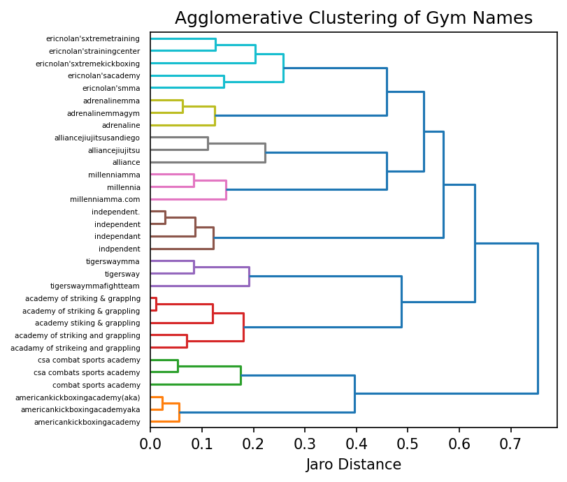
A dendrogram illustrating the results of agglomerative clustering by Jaro similarity on a subset of the gym names.

The object returned by AgglomerativeClustering() includes the cluster labels for each item, which I append to my dataframe as the column gym_cluster_labels.

df['gym_cluster_labels'] = clustering.labels_
df.head()

name	age	weight	gym	city	mma_w	mma_l	mma_total	gym_cluster_labels
Gabriella Sullivan	26	Flyweight - 115.1 to 125 pounds	Azteca	Lakeside	0	1	1	1255
Jeremiah Garber	27	Lightweight - 145.1 to 155 pounds	10th Planet HQ - The Yard	Los Angeles	0	1	1	324
Rodrigo Oliveira	32	Lightweight - 145.1 to 155 pounds	Triunfo Jiu-jitsu & mma	Pico Rivera	1	0	1	206
Ronell White	20	Lightweight - 145.1 to 155 pounds	Team Quest	Oceanside	0	1	1	719
Enrique Valdez	22	Middleweight - 170.1 to 185 pounds	Yuma top team	Yuma	1	0	1	785

Now with reliable labels, it becomes possible to aggregate and get descriptive statistics. A natural question may be: how successful are the largest gyms? This code returns g as a dataframe containing the name, total mma fight count and win rate of each gym:

g = df.groupby(['gym_cluster_labels']).agg(
        gym_name = pd.NamedAgg('gym', lambda x: x.iloc[0]), #use the first gym name in the cluster as a representative, for readability
        N_wins = pd.NamedAgg('mma_w', 'sum'),
        N_total = pd.NamedAgg('mma_total', 'sum'))

Note: NamedAgg() returns g as a single-indexed dataframe, which will be easier to query later. It can be thought of as a drop-in replacement for SQL AS.

To improve readability, I modify the styler object corresponding to g so that the win rate cell is colored in proportion to its value.

s = g.sort_values(by='N_total', ascending=False).iloc[0:10,:].style
s.format(precision=2)
s.background_gradient(cmap='RdYlGn',vmin=0, vmax=1, subset=['win_rate'], axis=1)

Here is a look at the 10 largest gyms in the dataset:

gym_name	N_wins	N_total	win_rate
Independent	289	880	0.33
Team Quest	181	355	0.51
DragonHouse MMA	101	215	0.47
Millennia	125	203	0.62
The Arena	131	202	0.65
Team Alpha Male	115	167	0.69
Bodyshop	86	153	0.56
CSW	88	145	0.61
CMMA	86	142	0.61
Victory MMA	82	130	0.63

According to the data, the largest “gym” is actually the group of fighters with no gym affiliation. This group performs notably worse than the next largest gyms. This may imply that the benefits of belonging to a gym – coaching, infrastructure, training partners – have an effect on fighter outcomes. Alternatively, good fighters may be seeking out the best gyms and vice-versa. It is difficult to infer causality without individual fight and gym affiliation information as a function of time.

The tabular representation is fine for a few rows of information, but quickly becomes overwhelming as the data grow larger.

Geospatial Visualization

A good visualization of large, multi-dimensional data is one that compresses multiple features into a relatively small number of plotted objects in an appealing way, without sacrificing information content. In this case, I use geography as the foundation to build a global visual representation of the data.

Geopy

First, I had to geocode the data – i.e., convert a list of gym names into map coordinates. GeoPy is a python library which allows a user to query the API of a variety of geocoding services. I used Google’s geocoding API, which is not free in general, but allows a certain number of free queries per month.

I query the API sequentially with every gym name in a given cluster until I get the coordinates for that gym, then go to the next cluster. This is a lazy way to to avoid excessively redundant calls to the API. The returned object is a geopy.Point() containing a latitude and longitude.

#a null column to populate with coordinates
g['gym_lat'] = pd.NA
g['gym_lon'] = pd.NA

from geopy.geocoders import GoogleV3
geolocator = GoogleV3(api_key='<MY_API_KEY>')

from geopy.extra.rate_limiter import RateLimiter
geocode = RateLimiter(geolocator.geocode, min_delay_seconds=1, max_retries=1, error_wait_seconds=10)

for gcl in g.index:
      gym_group = df[(df['gym_cluster_labels'] == gcl)]['gym']

      for gym_name in gym_group:
          location = geocode(query=gym_name, components=[('administrative_area', 'CA'), ('country', 'US')])

          #filter out null and default response from API
          if (location is not None) and (location.raw['place_id'] != 'ChIJPV4oX_65j4ARVW8IJ6IJUYs'):
              g.loc[gcl, 'gym_lat'] = location.latitude
              g.loc[gcl, 'gym_lon'] = location.longitude
              break

Sidenote: Setting up the Geocoding API

On GCP, geocoding is handled by the Geocoding API. To access the API, you have to first generate an API key. From the cloud console dashboard, enter the navigation menu, then go to APIs & Services → Credentials

On the top of the Credentials page, click the Create Credentials button and select API key from the dropdown menu. The new key will show up on your credentials dashboard. In the row with the newly created key, select Actions → Edit API Key. Under API restrictions, select Restrict Key, then in the dropdown menu, check the Geocoding API and OK.

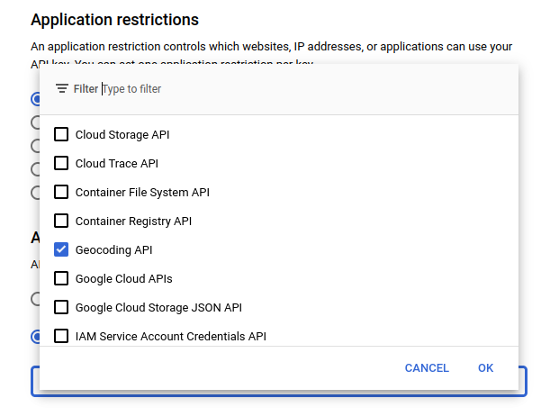
Now if you click SHOW KEY on the credentials dashboard, you’ll see the alphanumeric string you need to pass to geopy to authenticate the calls to the API.

Warning: The API key is linked to your billing account, so keep it protected!

Folium

With the geocoded data, I generated an interactive map of the MMA gyms across California with Folium, a python wrapper for leaflet.js. First, I generate the folium.Map object with a default map center and starting zoom value. Then, I define a RGBA colormap to color the map markers. Each marker is a circle centered on a gym location, with its size and color corresponding to the gym’s total fight count and win rate, respectively. The unaffiliated fighters are represented by a marker placed off the coast of Santa Cruz:

marker_data = g
marker_data.loc[413, 'gym_lon'] = -125. #shift the 'Independent' entry

import folium
ca_coordinates = (37.41928,-119.30639)
map = folium.Map(location=ca_coordinates,
                 zoom_start=6,
                 max_zoom=9,
                 tiles='cartodb dark_matter')

import branca.colormap as cm
#Red-White-Green colormap
gradient = cm.LinearColormap([(255,0,0,255), (255,255,255,125),(0,255,0,255)],
                              vmin=0., vmax=1.,
                              caption='win rate')

for idx,row in marker_data.iterrows():
    folium.Circle(
        location=[row.gym_lat, row.gym_lon],
        radius=row.N_total*100,
        weight=0, #stroke weight
        fill_color= gradient.rgba_hex_str(row.win_rate),
        fill_opacity=gradient.rgba_floats_tuple(row.win_rate)[-1]
    ).add_to(map)

map.add_child(gradient)

map

A map of MMA gyms in California. The size of each marker is scaled to the total number of fights of the gym, and the color corresponds to the percentage of fights won. The unaffiliated fighters are aggregated into a single marker shown off the coast of Santa Cruz.

If you are curious about the thumbnail image for this project, see here

MMA Gym Analysis

Arjun Rana