
NOTE: The accompanying code for this project can be found here
Summary
In this project, I am provided with a minimal dataset containing locations and sizes of self-storage facilities across the country. The objective is to identify demographic variables that influence the self-storage market. Using data from the American Community Survey, I perform non-parametric robust regression to identify key factors that influence self-storage demand. I also explain and demonstrate the importance of choosing an optimization scheme that matches the business context of a problem. I conclude with a geospatial visualization of the results and a recommendation of specific regions with high unmet demand.
Intro
Self storage is an expansive, multi-billion dollar industry utilized by 1 in 11 Americans (ref). In contrast to residential real-estate, self-storage is a relatively stable investment as indicated by a low SBA loan default rate (ref). Major industry players compete for control of metropolitan areas due to their high profitability. In this case study, a self-storage company gives me a .csv containing locations and square footage of self-storage facilities with an open-ended objective: explore demographic trends that influence the self-storage market and provide recommendations for investment strategy to the company.
| Market | Owner/Operator, Franchise | ADDRESS | CTY | ST | Zip | Area | Year | |
|---|---|---|---|---|---|---|---|---|
| 0 | Albuquerque | ##### | ##### | Santa Fe | NM | 87505 | 73934 | 2000 |
| 1 | Albuquerque | ##### | ##### | Rio Rancho | NM | 87124 | 72836 | 2000 |
| 2 | Albuquerque | ##### | ##### | Albuquerque | NM | 87114 | 80889 | 1998 |
| 3 | Albuquerque | ##### | ##### | Albuquerque | NM | 87111 | 62697 | 1997 |
| 4 | Albuquerque | ##### | ##### | Albuquerque | NM | 87114 | 60821 | 1998 |
Scenarios like this are an accurate representation of real-world data science where a solution involves business context, messy data from multiple sources and a healthy amount of trial and error. Market strategy is complex, dynamic system involving expansion, contraction and homeostasis, so the first step is to form a quantitative problem statement. My plan was to find localized demographic data and perform regression to a demand metric that I derived from the given data.
Model Selection
Gradient-boosted decision trees(GBDT) are the state-of-the-art in regression/classification tasks on structured data, as demonstrated by the sustained popularity of libraries like XGBoost and LightGBM (ref). I used LightGBM with 3-fold cross validation for all the results shown in this project.
Modeling Demand
One challenge faced in this project is to model demand from the given data, which contains no direct measure of demand. According to financial models of self-storage, cash flow for a facility is simply proportional to its square footage, so an approximation of the realized demand for a given geographical region $A$ can be modeled as
\[D_{A} = \sum_{i \in A} S_i\]where $S_i$ is the leasable square footage of facility $i$ in region $A$ (ref). This simple model assumes a national average rental price.
There are many different geographical areas defined by the census bureau. While zip codes offer granularity, core based statistical areas(CBSAs) are more useful from a business perspective because they indicate areas of high population density and economic activity. So, the demand target was modeled as an aggregation over CBSAs. A crosswalk table provided by the Department of Housing and Urban Development was used to convert zip codes to CBSAs (ref).
Demographic Data
The demographic data was collected from the American Community Survey(ACS), which contains detailed demographic information about housing, employment and education. The following code snippet was used to download the data:
NOTE: Use of the census API requires an API key
import requests
import pandas as pd

with open('API_census.txt') as key:
    API_KEY = key.read()

    def get_acs5_2020_group(group):

        year_='2020'
        source_='acs'
        name_='acs5' #5 year estimates
        table_='profile' #[detailed, subject, profile]
        base_ = f'https://api.census.gov/data/{year_}/{source_}/{name_}/{table_}'
        geog_type = 'metropolitan%20statistical%20area/micropolitan%20statistical%20area'
        data = requests.get(f'{base_}?get=group({group})&for={geog_type}:*&key={API_KEY}')
        data = data.json()
        acs_data=pd.DataFrame(data[1:], columns=data[0]).set_index(' '.join(geog_type.split(sep='%20')))

        #only keep 'estimates' cols
        acs_data = acs_data.filter(regex='\dE$', axis=1)
        return acs_data

      group_list = ['DP03', 'DP04', 'DP05']
      acs = []

      for group in group_list:
          acs_ = get_acs5_2020_group(group)
          acs.append(acs_)

      acs = pd.concat(acs, axis=1)
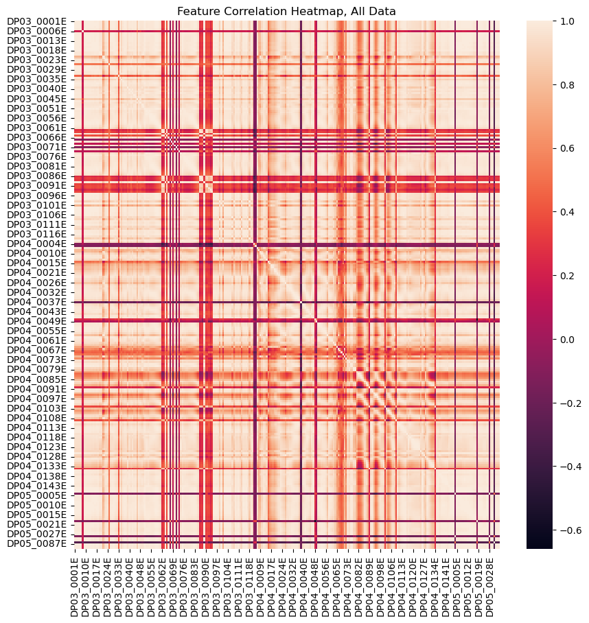
The ACS variables are grouped by conceptual similarity and labeled with a DP prefix. Group DP03 is a collection of economic characteristics, DP04 contains housing characteristics and DP05 includes age demographics by household (ref). The full dataset is highly degenerate, as shown by the correlation heatmap. The presence of many correlated features in the training data can make a model less interpretable and introduces numerical instability.
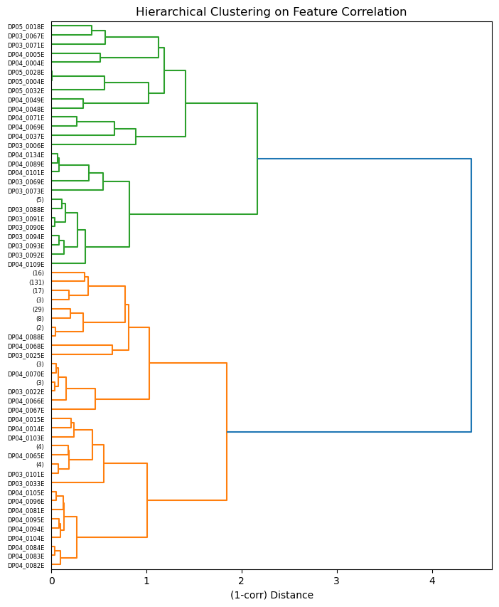
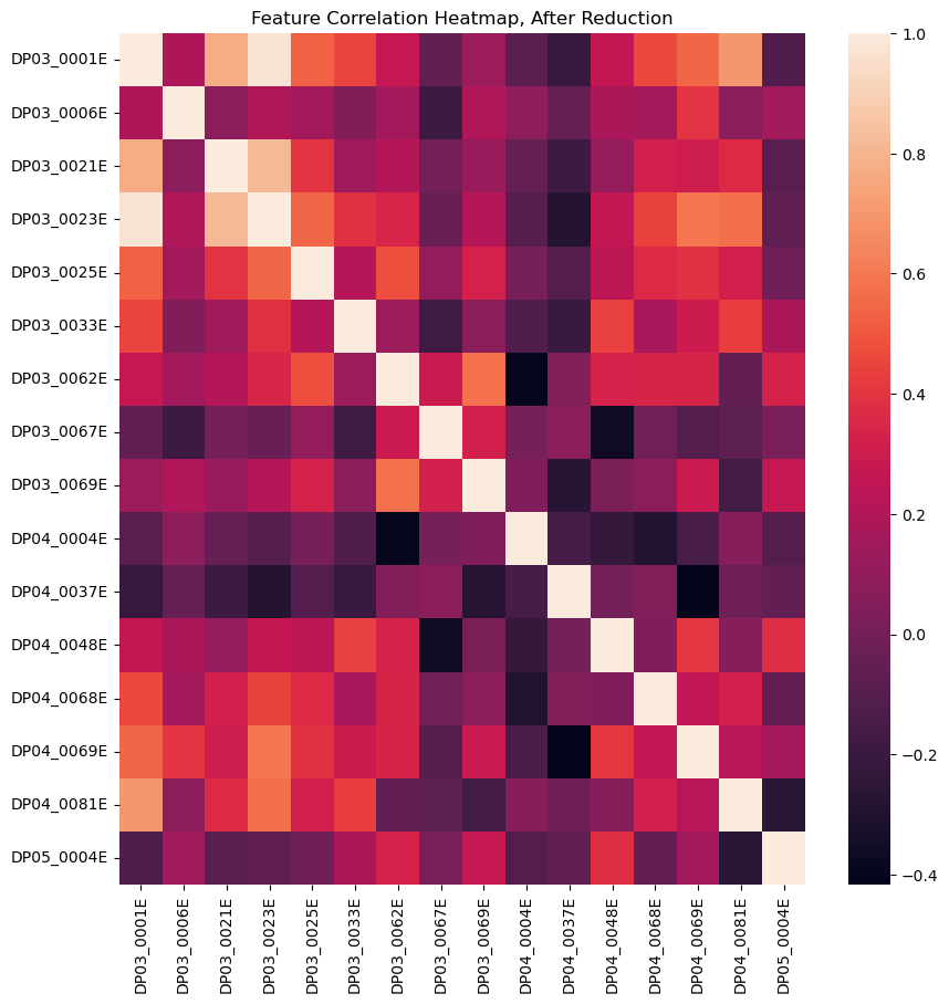
For a group of correlated features, one remedy is to drop all but one of the correlated features, which also decreases the dimensionality of the data and improves computational performance. With correlation as a distance metric, hierarchical clustering is used to aggregate similar features into groups. The total number of clusters is determined by a distance threshold heuristic, and a single feature from each cluster is included in the training data.
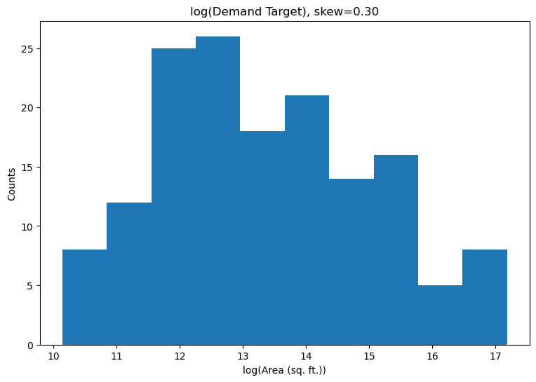
Target Skew and Business Context
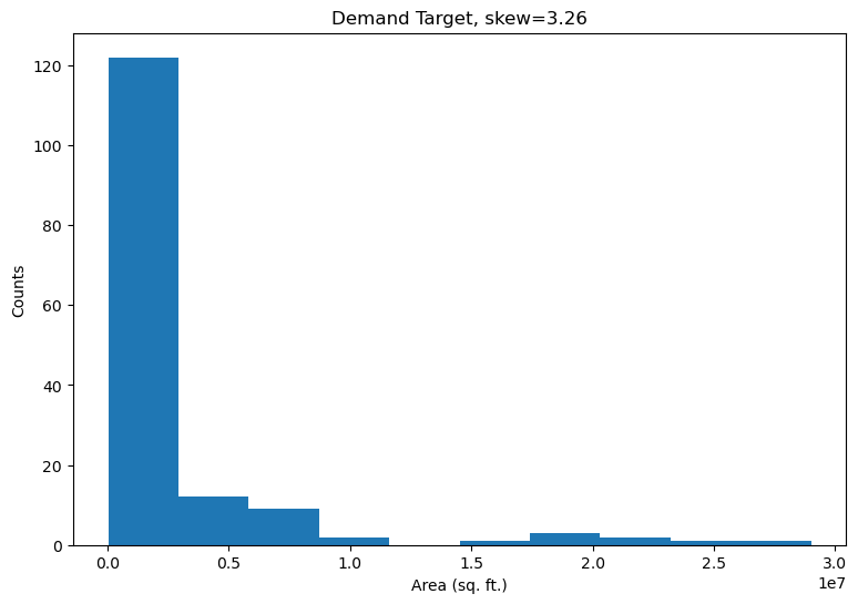
The target distribution is right-skewed because the majority of CBSAs fall into the low demand range with a few extreme exceptions. The conventional approach is to reduce the effect of outliers, so that the model more accurately reflects the statistics of the bulk population. In this case, the business objective is to target regions with high demand for expansion, so regression accuracy of the outliers needs to be a top priority. The two examples below illustrate how some conventional techniques fail from a business standpoint.
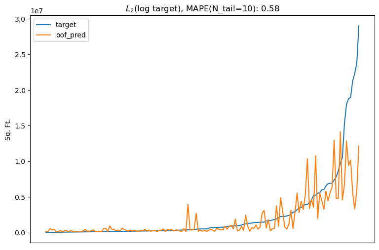
One common way to deal with skew is to $log$ transform the target, then do regression and exponentiate the model output for prediction (ref). The underlying assumption is that the target empirically fits a $log-normal$ distribution, so taking the $log$ results in normal distribution.
This approach can improve the quality of fit for points near the mean, but it comes at the cost of tail points–taking the $log$ reduces variance of the target by pulling outliers closer to the mean and thus reducing their importance. Additionally, the $log$ is a non-affine transformation under $L_2$ minimization (ref). This means taking the exponential of output produced by an $L_2$ minimizer trained on the $log$ target does not strictly correspond to the expected value of the target. Considering most software libraries use $L_2$ as the default regression objective, this would require the addition of a correction factor to the model output, introducing unnecessary complexity to the code.
Even without transforming the target, $L_2 = (y-\hat y)^2$ is not a good metric for this problem because it is sensitive to absolute error. For example, using $L_2$ implies a 2,000 sq. ft. demand estimate of a 1,000 sq. ft. target is just as wrong as a 101,000 sq. ft. estimate of a 100,000 sq. ft. target.
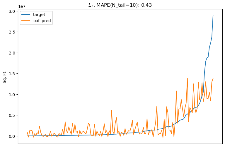
The specific business context of this problem clearly calls for a relative metric that scales with target value, making it robust to extreme values.
Tweedie: A Robust Regression Metric
The Tweedie distribution is a generalized exponential probability distribution that encompasses the normal, Poisson, and gamma distributions, among others. A random variable $Y$ is Tweedie distributed if the mean-variance relationship follows the power relationship
\[Var(Y) = \phi \mu^\rho\]where $\phi$ is a dispersion term and $\rho$ is the power parameter. The mean-variance relationship can be used to derive the probability density function (ref). Strictly positive, right-skewed distributions like the self-storage demand target can be modeled by a Tweedie distribution where $ 1 < \rho < 2$ and $\mu > 0$. The likelihood loss function can be derived (ref):
\[L(y_i, \hat y_i \vert \rho) = -\frac{y_i e^{(1-\rho)\hat y_i}}{1-\rho} + \frac{e^{(2-\rho)\hat y_i}}{2-\rho}\]Consequently, the optimal tree splits are determined iteratively via the gradient
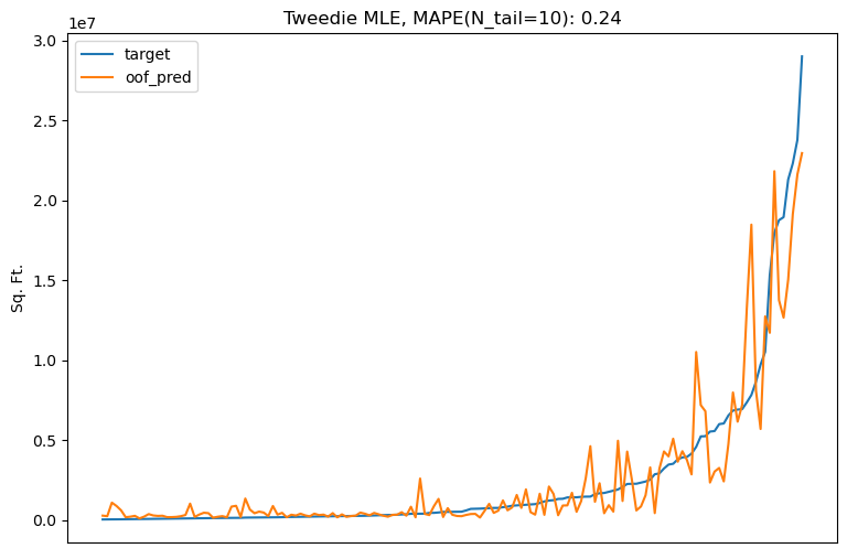
\[\frac{\partial L}{\partial \hat y_i} = -y_i e^{(1-\rho)\hat y_i} + e^{(2-\rho)\hat y_i}\]As shown in the animation below, Tweedie loss in this power regime penalizes outliers less severely than $L_2$ loss, and the penalty can be tuned via the power parameter.
The flexibility and robustness of Tweedie loss make it a good match for the business needs of the problem. Replacing the $L_2$ objective with an appropriately tuned Tweedie objective decreases tail prediction error by nearly a factor of 2, from 43% to 24% MAPE.
Feature Selection
Feature selection is used to understand which features contribute most to a fitted estimator’s predictions. This is not only important to explainability, but is also used to reduce the number of input variables and improve computational performance at scale. Quantifying feature importance in decision tree based models is relatively straightforward: split importance is a count of how often a feature is used to split the data, gain importance is a measure of reduction in error from splits where a specific feature is used (ref).
It is important to normalize feature importance to eliminate bias. Null feature importance is one approach to normalization in which the model is repeatedly re-trained with a randomly shuffled target variable (ref). Target shuffling generates a null distribution of importance for each feature to serve as a baseline. Features are important only if the true importance is sufficiently separated from the null distribution. While this technique is computationally intensive, it is model agnostic and reliable. The results shown here are with a null distribution of 100 runs. Features were classified as important if the true importance was greater than the median of the null distribution. Both gain and split importance were measured for all features.
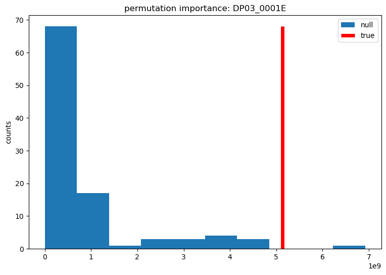
DP03_0001E is a count of the employed population, aged 16 and over. This is an example of a feature that is important to the model, where the true value is above the null median.
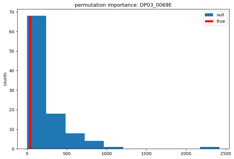
DP03_0069E is the mean retirement income of households with retirement income. This is an example of a feature that is unimportant to the model, where the true value is below the null median.
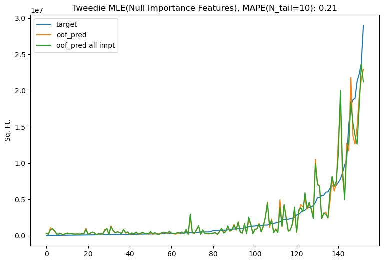
The final model is re-trained using only the important features. Removing extraneous features improves the tail error to 21%.
Predictions
Out of the 939 CBSAs defined in the US Census, the training dataset contains 153 unique CBSAs. I assume that it is a complete list and use the remaining 786 CBSAs to generate predictions for self-storage demand. Regions with a high predicted target score are interpreted as those that can sustain a larger self-storage market. The result can be clearly explained (i.e. in a meeting with non-technical stakeholders) with a choropleth map. The interactive map shown below shows the predicted demand for all CBSAs that were not in the training data, with deeper green corresponding to a higher predicted demand score. According to the model, some regions with notable predicted demand include Edinburg(TX), Boise(ID) and Madison(WI). A targeted expansion in these three areas alone could generate $10M in annual pre-tax cash flow.