
Summary
I use Google BigQuery to engineer and analyze purchasing data from Iowa’s largest liquor stores. A forecasting model is trained on this data to infer future store sales and demand for inventory. I conclude with an overview of cloud-native solutions to serve and maintain the trained model.
BigQuery
BigQuery(BQ) is a SQL-centric data warehouse sold by Google Cloud Platform (GCP). It is primarily used for storage and ad-hoc analysis of structured data that can be ingested from a variety of sources. BQ’s value proposition is based on performance – high throughput, low latency data processing is achieved through a decoupling of the storage and computation frameworks.
BigQuery ML(BQML) is BigQuery’s native machine learning functionality. The appeal of BQML is apparent when the training data is already stored in BQ, as developing a model is a matter of a few SQL commands. While ultimate accuracy may require training a custom model, BQML produces good results at a fraction of the time and cost.
Data Exploration
To attract users, GCP hosts a variety of datasets that can be explored with their products. I was interested in the retail sector, so I chose to look at data provided by the Iowa Dept. of Commerce. The dataset contains all the wholesale liquor purchases made by liquor stores across Iowa, from January 2012 onwards. At the time of writing, the table contains ~24 million sales records. The schema is:
| Column Name | Description | Data Type |
|---|---|---|
| invoice_and_item_number | Concatenated invoice and line number associated with the liquor order. This provides a unique identifier for the individual liquor products included in the store order | STRING |
| date | Date of Order | DATE |
| store_number | Unique number assigned to the store who ordered the liquor | STRING |
| store_name | Name of store who ordered the liquor | STRING |
| address | Address of store who ordered the liquor | STRING |
| city | City where the store who ordered the liquor is located | STRING |
| zip_code | Zip code where the store who ordered the liquor is located | STRING |
| store_location | Location of store who ordered the liquor. The Address, City, State and Zip Code are geocoded to provide geographic coordinates. Accuracy of geocoding is dependent on how well the address is interpreted and the completeness of the reference data used | STRING |
| county_number | Iowa county number for the county where store who ordered the liquor is located | STRING |
| county | County where the store who ordered the liquor is located | STRING |
| category | Category code associated with the liquor ordered | STRING |
| category_name | Category of the liquor ordered | STRING |
| vendor_number | The vendor number of the company for the brand of liquor ordered | STRING |
| vendor_name | The vendor name of the company for the brand of liquor ordered | STRING |
| item_number | Item number for the individual liquor product ordered | STRING |
| item_description | Description of the individual liquor product ordered | STRING |
| pack | The number of bottles in a case for the liquor ordered | INT |
| bottle_volume_ml | Volume of each liquor bottle ordered in milliliters | INT |
| state_bottle_cost | The amount that Alcoholic Beverages Division paid for each bottle of liquor ordered | FLOAT |
| state_bottle_retail | The amount the store paid for each bottle of liquor ordered | FLOAT |
| bottles_sold | The number of bottles of liquor ordered by the store | INT |
| sale_dollars | Total cost of liquor order (number of bottles multiplied by the state bottle retail) | FLOAT |
| volume_sold_liters | Total volume of liquor ordered in liters (i.e. (Bottle Volume (ml) x Bottles Sold)/1,000) | FLOAT |
| volume_sold_gallons | Total volume of liquor ordered in gallons (i.e. (Bottle Volume (ml) x Bottles Sold)/3785.411784) | FLOAT |
I wanted to investigate some fundamentally relevant business problems that fall within the scope of machine learning – forecasting store activity and predicting demand for specific goods. A reliable prediction of store activity can be used to distribute personnel, produce targeted marketing and detect anomalies. Forecasting demand for specific products can be useful for optimization of ordering/shipping and to mitigate the risk of stockouts.
I began by exploring the data manually, starting with identification of the largest stores:
SELECT
  store_name,
  ANY_VALUE(store_number) AS store_id,
  COUNT(invoice_and_item_number) AS order_count
FROM
  `bigquery-public-data.iowa_liquor_sales.sales`
GROUP BY
  store_name
ORDER BY
  order_count DESC
LIMIT
  10
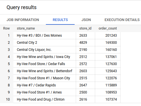
The query results show that Hy-Vee in Des Moines is the most active store by a considerable margin, with over 200k orders. The top 10 largest stores all have over 100k orders. Later, the store_id field will make it easy to aggregate the training and testing data for the forecasting model. I isolated Hy-Vee to get a sense of the the order count for different types of alcohol:
SELECT
  ANY_VALUE(category_name),
  COUNT(invoice_and_item_number) AS order_count,
  category
FROM
  `bigquery-public-data.iowa_liquor_sales.sales`
WHERE
  store_number = '2633'
GROUP BY
  category
ORDER BY
  order_count DESC
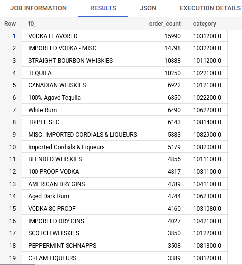
I noticed I could bin the orders by the first three digits of the category code as a good approximation of store inventory by type.
Machine Learning
BQML only works on structured data (look at autoML for image/video data) when the machine learning task is one of: linear/logistic regression, DNN classification, xgboost classification/regression, k-means clustering, dimensionality reduction (PCA, autoencoder), matrix factorization or forecasting. I want to infer future values based on historical trends, so a forecasting model is the appropriate choice.
ARIMA: A Forecasting Model
For forecasting, BQML implements a model called ARIMA. ARIMA is a generalization of ARMA, a model comprised of an autoregressive and moving-average component:
\[X_t(p,q) = c + \epsilon_t + \sum_{i=1}^{p}\phi_i X_{t-i} + \sum_{i=1}^{q} \theta_i \epsilon_{t-i}\]In this model, \(p\) is the order of previous time steps in the autoregression and \(q\) is the order of previous time steps in the moving-average. ARIMA is similar to ARMA, but computed on the difference up to order \(d\). For example:
\[X_{d=1} = X_t - X_{t-1}\] \[X_{d=2} = (X_t - X_{t-1}) - (X_{t-1} - X_{t-2})\]and so on.
Then, the ARIMA model looks like
\[X_{d}(p,d,q) = c + \epsilon_t + \sum_{i=1}^{p}\phi_i X_{d-i} + \sum_{i=1}^{q} \theta_i \epsilon_{t-i}\]When training an ARIMA model, BQML searches for the best \(p,d,q\). I will end the discussion of the model here, as there is a lot of well-written information available online.
Data Formatting
I created two tables: one for large store activity and the other for inventory at the largest store. Table #1 contains the dollar value of orders placed by the 10 largest stores, aggregated by month. I assume that liquor is sold only by the store which ordered it, and that store-to-store transfer of inventory isn’t allowed, so I call this aggregate monthly_sales_total.
NOTE: I replaced my actual project and dataset names with my-project and my-dataset
CREATE OR REPLACE TABLE
  `my-project.my-dataset.top10_monthly_bqML_train` (date_trnc DATE, store_number STRING, monthly_sales_total FLOAT64)
AS SELECT
  DATE_TRUNC(date, MONTH) AS date_trnc,
  store_number,
  SUM(sale_dollars) AS monthly_sales_total
FROM
  `bigquery-public-data.iowa_liquor_sales.sales`
WHERE
  date BETWEEN DATE('2012-01-01') AND DATE('2019-12-31')
  AND
  store_number IN ('2633', '4829', '2190', '2512', '2572', '2603', '2515', '2647', '2500', '2616')
GROUP BY
  date_trnc, store_number
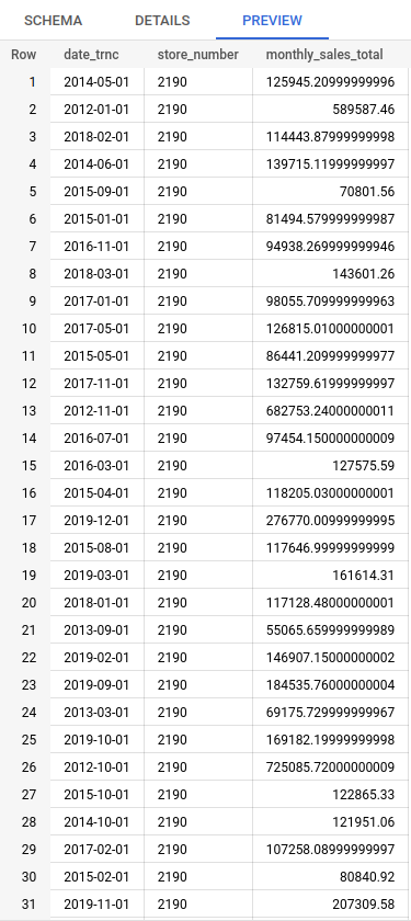
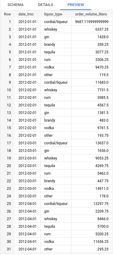
Table #2 contains the volume of liquor ordered by Hy-Vee in Des Moines, aggregated into the most common types. The volume metric could be used to predict demand and mitigate stockouts or excessive purchases. The category is determined from the prefix of the category code.
CREATE OR REPLACE TABLE
  `my-project.my-dataset.store2633_monthly_liquor_types_bqML_train` (date_trnc DATE, liquor_type STRING, order_volume_liters FLOAT64)
AS SELECT
  DATE_TRUNC(date, MONTH) AS date_trnc,
  CASE
    WHEN STARTS_WITH(category, '101') THEN 'whiskey'
    WHEN STARTS_WITH(category, '102') THEN 'tequila'
    WHEN STARTS_WITH(category, '103') THEN 'vodka'
    WHEN STARTS_WITH(category, '104') THEN 'gin'
    WHEN STARTS_WITH(category, '105') THEN 'brandy'
    WHEN STARTS_WITH(category, '106') THEN 'rum'
    WHEN STARTS_WITH(category, '108') THEN 'cordial/liqueur'
    ELSE 'other'
    END
    AS liquor_type,
  SUM(volume_sold_liters) AS order_volume_liters,
FROM
  `bigquery-public-data.iowa_liquor_sales.sales`
WHERE
  store_number = '2633' AND
  date BETWEEN DATE('2012-01-01') AND DATE('2019-12-31')
GROUP BY
  date_trnc, liquor_type
ORDER BY
  date_trnc ASC
Monthly aggregation was chosen for a few reasons. The data without aggregation is noisier, making it more difficult to clearly model trends. Training a model to output daily/weekly predictions could be too fast to adjust business decisions. On the other hand, a quarterly/yearly aggregation would be too slow. Data prior to 2020 was used for training because I wanted the forecast interval to include the early parts of the covid pandemic.
Training
Training a model in BigQuery ML is accomplished by calling CREATE MODEL. For table #1, this looks like:
CREATE OR REPLACE MODEL
  `my-dataset.top10_arima_model`
OPTIONS(
  MODEL_TYPE = 'ARIMA_PLUS',
  TIME_SERIES_TIMESTAMP_COL = 'date_trnc',
  TIME_SERIES_DATA_COL = 'monthly_sales_total',
  TIME_SERIES_ID_COL = 'store_number') AS
SELECT
  date_trnc, monthly_sales_total, store_number
FROM
  `my-project.my-dataset.top10_monthly_bqML_train`
The OPTIONS specify model input parameters, which are mostly self-explanatory. The TIME_SERIES_ID_COL is an optional parameter used to distinguish row ownership when multiple time series are being forecast concurrently.
Inference
After training is done, inferences are drawn from the model using the appropriate inference function. ARIMA uses ML.FORECAST and returns a forecast that is 3 time points long by default
SELECT
  store_number,
  FORMAT_TIMESTAMP("%Y-%m-%d", forecast_timestamp) AS date_trnc,
  forecast_value AS monthly_sales_forecast,
  prediction_interval_lower_bound,
  prediction_interval_upper_bound
FROM
  ML.FORECAST(MODEL `my-project.my-dataset.top10_arima_model`)
Results (Google Data Studio)
I visualized the results using Data Studio. Some functionality is lacking, but it wins for ease-of-use if your data lives within the GCP ecosystem. I connected the BQ output directly to Data Studio, so the visualizations update alongside the data.
There was no good way to display error bars, so I generated composite bar/line graphs. Each 4-page report contains the three month forecast and an error page. Each forecast (orange line) is shown with the upper and lower bounds of the 95% confidence interval (magenta and cyan lines) and compared against the true values (bars).
The sales forecast for the 10 largest stores:
The inventory forecast for the largest store:
The error page shows the mean absolute error percentage of each forecast from the true value. This report is interactive, so you can click any store number or alcohol type and see the corresponding percentage error per month. There is a relatively large forecast error in March as compared to January and February, most likely caused by the covid pandemic.
Excluding March, the forecast results for most stores and inventory are reasonable (<10% APE). Depending on business criteria, these results could be used directly or serve as a baseline for further optimization with more specific goals.
MLOps
In a business setting, model training is a relatively small part of the machine learning pipeline. The overhead associated with MLOps is significant and needs to be accounted for during the pipeline building phase.
One important aspect of MLOps is serving the model after training. For the model trained in this project, a ML.FORECAST query can be used to define a view that connects to a business intelligence tool for visualization and reporting. This allows for easy distribution of model inferences in an intuitive format, while still controlling access to the underlying data. If low latency or streaming is a requirement, the trained model can be exported as a Tensorflow SavedModel and deployed to a Vertex AI endpoint.
Also consider that trends in the data may change over time, in which case the model will need to be re-trained. The Iowa liquor store data updates monthly, so a scheduled query with a sliding time window would be a simple way to handle model re-training. Perhaps the data updates irregularly, or we want to minimize training costs by only re-training when an error metric exceeds an acceptable value. A Cloud Function could be written to trigger re-training based on a data update or model evaluation event. In a general E-T-L pipeline, model training can depend on output from various upstream components. Orchestration of the entire pipeline can be managed with Cloud Composer.